
For more complicated programs it is not easy to determine the number of independent paths of the program. McCabe’s cyclomatic complexity defines an upper bound for the number of linearly independent paths through a program. Also, the McCabe’s cyclomatic complexity is very simple to compute. Thus, the McCabe’s cyclomatic complexity metric provides a practical way of determining the maximum number of linearly independent paths in a program. Though the McCabe’s metric does not directly identify the linearly independent paths, but it informs approximately how many paths to look for.
There are three different ways to compute the cyclomatic complexity. The answers computed by the three methods are guaranteed to agree
Method 1:
Given a control flow graph G of a program, the cyclomatic complexity V(G) can be computed as:
V(G) = E – N + 2
where N is the number of nodes of the control flow graph and E is the number of edges in the control flow graph.
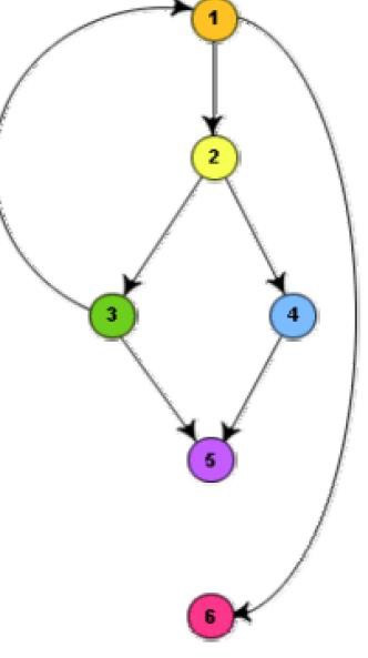
For the CFG of above diagram , E=7 and N=6. Therefore, the cyclomatic complexity = 7-6+2 = 3.
Method 2:
An alternative way of computing the cyclomatic complexity of a program from an inspection of its control flow graph is as follows:
V(G) = Total number of bounded areas + 1
In the program’s control flow graph G, any region enclosed by nodes and edges can be called as a bounded area. This is an easy way to determine the McCabe’s cyclomatic complexity.
But, what if the graph G is not planar, i.e. however you draw the graph, two or more edges intersect? Actually, it can be shown that structured programs always yield planar graphs. But, presence of GOTO’s can easily add intersecting edges. Therefore, for non-structured programs, this way of computing the McCabe’s cyclomatic complexity cannot be used.
The number of bounded areas increases with the number of decision paths and loops. Therefore, the McCabe’s metric provides a quantitative measure of testing difficulty and the ultimate reliability. For the CFG example shown in above fig, from a visual examination of the CFG the number of bounded areas is 2. Therefore the cyclomatic complexity, computing with this method is also 2+1 = 3. This method provides a very easy way of computing the cyclomatic complexity of CFGs, just from a visual examination of the CFG. On the other hand, the other method of computing CFGs is more amenable to automation, i.e. it can be easily coded into a program which can be used to determine the cyclomatic complexities of arbitrary CFGs.
Method 3:
The cyclomatic complexity of a program can also be easily computed by computing the number of decision statements of the program. If N is the number of decision statement of a program, then the McCabe’s metric is equal to N+1.